A More Efficient Digital Resonator
In previous posts, I described my digital resonator model: the main principles in Digital Resonator; a few more geeky details in Digital Resonator (II).
I have now understood how the way phase is handled in the FFT algorithm applies to the time domain. I knew it relies only in sine and cosine (via complex numbers), but I never came across an explanation that would help me understand it well enough. In this post I attempt to give an intuitively comprehensible explanation and outline the implications for my resonator model.
In Digital Resonator (II), I described the amplitude update computations for my resonator model as follows:
The resonator’s amplitude is updated at each tick of the clock, i.e. for each input sample, from the resonator’s current amplitude value a (in [0,1]), its current position in the oscillation period (waveform value w, in [-1,1]), and the input sample value s (in [-1,1]):
a <- (1-k) * a + k * s * w
The instantaneous contribution of each input sample value to the amplitude is proportional to s * w, which intuitively will be maximal when peaks in the input signal and peaks in the resonator’s waveform are both equally spaced and aligned, i.e. when they have same frequency and are in phase.
In order to account for phase offset, the above calculation is performed for various phases, and the resonator’s amplitude is set to the maximum value across all phases. (emphasis added)
In essence, we are looking for the maximum contribution at the given frequency (dictated by the waveform), but don’t know the phase offset. We take the brute force approach of computing the contribution for many offsets, i.e. sampling the resulting curve at as many points as we can, and then take the maximum value.
This approach is less than satisfying as the complexity is linear in the number of phases, i.e. the number of samples in one period, which for low frequencies in the audible spectrum typically reaches a few thousands. It turns out that it is also completely unnecessary!
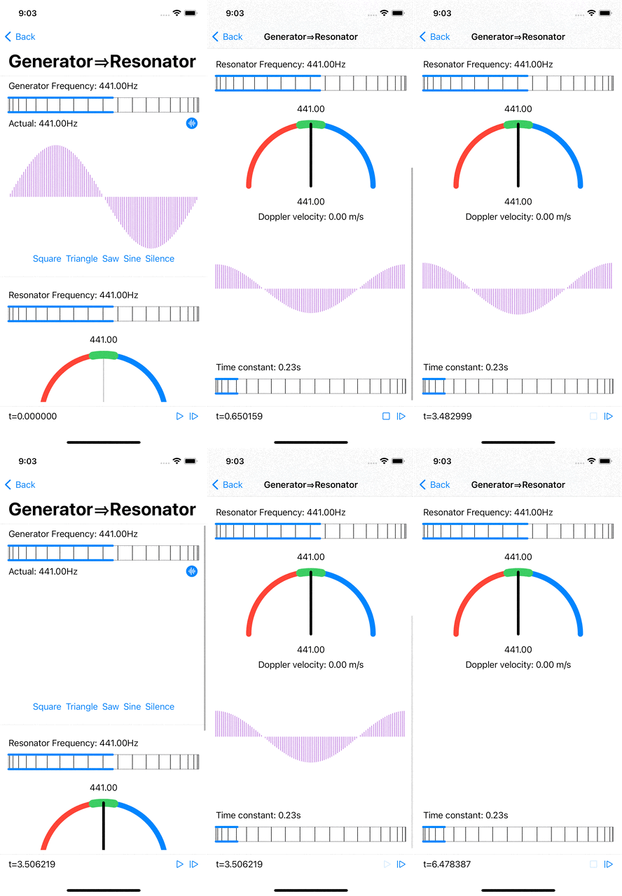
Here is what made the penny drop for me: suppose the waveform W is a sine curve, then the collection of instantaneous contributions for a given sample value s at each phase is also a (scaled) sine curve (s * W), and so are the accumulated amplitude values, as they are linear combinations of sines, all of the same frequency. The sine shape of the phases plot is quite obvious in the app screenshot below.

|
| The resonator's amplitudes (at all phases) increase when the generator produces a sinusoidal signal at the resonator's resonant frequency. The amplitude is maximal at the corresponding phase. |
We want to calculate the amplitude and phase offset of s * W, therefore we only need to compute and accumulate the signal’s contribution at 2 phase values (there are only 2 degrees of freedom!). For a sine waveform sin(x), the natural candidates are phases 0 and 𝜋/2, i.e. sin(x) and sin(x+𝜋/2) = cos(x).
This can be formulated and implemented neatly and compactly with complex numbers, but intuitively, instead of computing the amplitude at each phase, the resonator maintains two values, ps and pc (both in [0,1]), updated at each tick of the clock, i.e. for each input sample, from their current values, the current position in the oscillation period (values ws for the sine waveform and wc for the cosine waveform, both in [-1,1]), and the input sample value s (in [-1,1]):
ps <- (1-k) * ps + k * s * ws
pc <- (1-k) * pc + k * s * wc
These two values are two sample points on the “all phases” curve. At any tick, the resonator’s amplitude is sqrt(ps*ps + pc*pc) and the phase offset arctan(ps/pc).
This is of course a much more efficient way of implementing digital resonators: the number of computations required per update is much smaller than in the brute force approach, and is independent of the resonator’s frequency. This will certainly allow for resonator banks with more resonators. In addition, the approach of encoding a whole bank of oscillators as one array, with each update a single call to the Accelerate framework, is worth revisiting as it might prove more efficient than the “independent resonators” approach.